How to Properly Find Degrees of Freedom in Statistical Analysis

Understanding how to find degrees of freedom is crucial in statistical analysis. Degrees of freedom (DF) represent the number of values in a calculation that are free to vary. They are foundational to many statistical tests, including t-tests, ANOVA, and regression analysis. This article provides a detailed guide on calculating degrees of freedom across different types of statistical tests.

Understanding Degrees of Freedom in Statistics

The **degrees of freedom** in statistics reflect the number of independent pieces of information available to estimate a parameter. This concept is pivotal across various statistical methods, as it influences the behavior of statistical tests in determining outcomes such as p-values. For instance, in hypothesis testing, the correct calculation of degrees of freedom can directly impact **statistical significance**. Usually expressed as \( n – k \) (where \( n \) is the number of observations, and \( k \) is the number of parameters estimated), understanding this basic formula lays the groundwork for more complex scenarios.

Degrees of Freedom Formula

The general **degrees of freedom formula** varies by statistical test. For a one-sample t-test, the formula is \( DF = n – 1 \). In contrast, for two-sample t-tests for independent samples, it is calculated as \( DF = n_1 + n_2 – 2 \), where \( n_1 \) and \( n_2 \) represent the sample sizes. This distinction is critical because different analyses require unique formulas for accurate degrees of freedom calculations, thereby affecting the test’s reliability and the confidence in the resulting inferences.

Role of Degrees of Freedom in Hypothesis Testing

The role of degrees of freedom in hypothesis testing cannot be understated. They dictate the distribution of the test statistic under the null hypothesis and, consequently, the critical values used to determine statistical significance. For example, using the **degrees of freedom in t-tests**, one can consult t-distribution tables to ascertain the precise cut-off points at which the null hypothesis can be rejected. The interplay between **degrees of freedom** and statistical power further illustrates why they are fundamental to statistical methodologies.

Degrees of Freedom in Linear Models

In linear regression, **degrees of freedom** serve several purposes, including estimating model variability. DF is calculated as the difference between the number of observations (n) and the number of estimated parameters (p). Thus, in a linear model involving intercept and slopes, DF will typically be \( n – p \). This information is essential for understanding model fit and is a building block for more advanced analyses like ANOVA.

Degrees of Freedom in ANOVA

ANOVA, or Analysis of Variance, leverages **degrees of freedom** to compare multiple means. In a one-way ANOVA, the total DF is split into between-group and within-group categories. The **between-group degrees of freedom** are calculated as \( k – 1 \) (where \( k \) is the number of groups), and the **within-group degrees of freedom** is calculated as \( N – k \) (where \( N \) is the total number of observations). This distinction identifies the sources of variation, making it easier to assess group differences.

Calculating DF for Effects in ANOVA

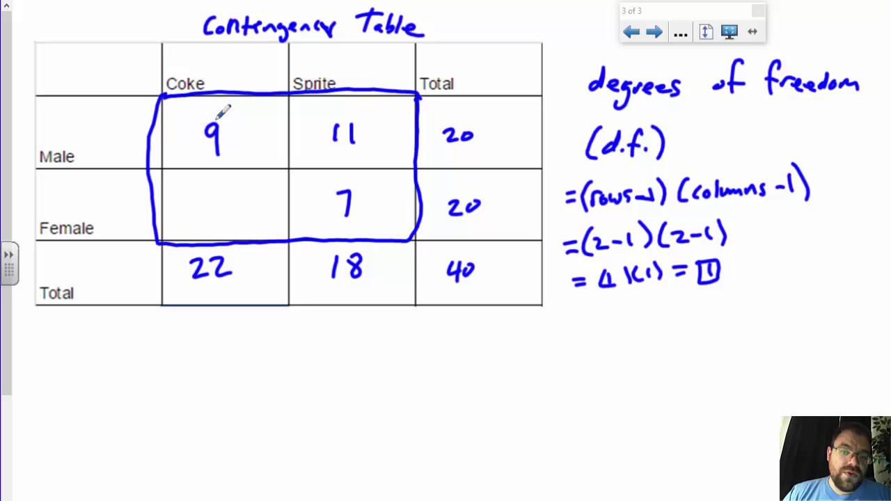
Within ANOVA, recognizing how to precisely calculate degrees of freedom for different effects is imperative. If there are two factors, such as in a two-way ANOVA, the DF can be categorized as follows: for Factor A, it’s \( a – 1 \); for Factor B, it’s \( b – 1 \); for interactions, it’s \( (a – 1)(b – 1) \). Such calculations ensure one can adequately interpret each term’s significance in the overall model.

Degrees of Freedom Adjustments

Sometimes adjustments need to be made to degrees of freedom to account for sample design intricacies or complex analytical frameworks. For example, in repeated measures ANOVA, the adjusted **degrees of freedom for paired samples** follow a different protocol based on the number of within-subjects degrees of freedom. Recognizing when and how to adjust degrees of freedom is essential in delivering accurate statistical outcomes and interpretations.

Degrees of Freedom in Regression Analysis

In regression analysis, understanding how degrees of freedom influences model evaluation is critical. **Degrees of freedom for residuals** are crucial for assessing the goodness of fit of the model. In a standard linear regression, the DF for residuals is calculated as \( n – p \), enabling the calculation of mean squares and F-statistics. This assessment is vital for scrutinizing the model’s effectiveness in explaining variance in the dependent variable.

Effect of Sample Size on Degrees of Freedom

The relationship between **sample size** and degrees of freedom is fundamental in regression analysis. Larger sample sizes generally increase degrees of freedom, which can enhance the accuracy of estimates and improve the model’s predictive power. However, overly large sample sizes can lead to detecting statistically significant results that may not be practically significant. Understanding this balance is essential for conducting meaningful analyses.

Statistical Power and Degrees of Freedom

The interaction between **degrees of freedom and statistical power** further elucidates the importance of correct calculations. More degrees of freedom increase the likelihood of identifying true effects in analyses, as greater freedom allows for a more nuanced investigation of statistical relationships. Researchers often strive to maximize degrees of freedom through optimal experimental design, emphasizing the significant role of degrees of freedom within statistical methodologies.

Practical Applications and Resources

To effectively apply the concepts surrounding **degrees of freedom** in real-world data analysis, it is beneficial to reference multiple **educational resources on degrees of freedom**. Websites with statistical tutorials and software documentation provide practical examples and case studies illustrating applications. Moreover, statistical software, such as R or Python libraries, often automates calculations for degrees of freedom, enhancing the accessibility and rigor of analysis without sacrificing accuracy.

Practical Examples of Degrees of Freedom

Visualizing **degrees of freedom in complex analyses** can significantly aid in statistical education. Consider a practical example involving ANOVA and regression. A one-way ANOVA analysis of agricultural yields from three different regions would show how to allocate degrees of freedom to between-group and within-group sums of squares effectively. The same principles apply in regression, where each coefficient estimated in the model consumes degrees of freedom, illustrating how dependencies shape estimations.

Using Degrees of Freedom in Statistical Software

Many statistical software packages take the burden of manually calculating degrees of freedom off the analyst. By inputting data correctly, users can easily fetch results that automatically include degrees of freedom calculations. This convenience not only streamlines the process but also aids in avoiding common errors associated with manual computations, emphasizing the importance of **using degrees of freedom in statistical software** for valid analyses.

Key Takeaways

• Degrees of freedom represent the flexibility of parameter estimation in statistical models.
• Accurate calculation methods depend on the statistical tests being executed, requiring knowledge of distinct formulas for each scenario.
• Understanding degrees of freedom improves the interpretation of statistical significance and overall model accuracy.
• Statistical software can simplify the calculation of degrees of freedom, enhancing efficiency and reducing human error.
• Proper consideration of degrees of freedom can significantly increase the power of hypothesis tests and foster better research outcomes.

FAQ

1. How do I calculate degrees of freedom for paired samples?

For paired samples, the degrees of freedom can be calculated using the formula \( n – 1 \), where \( n \) is the number of pairs. In hypothesis testing, correctly assessing the DF is crucial for the accuracy of significance results when comparing paired observations.

2. What are the implications of degrees of freedom in regression analysis?

In regression, degrees of freedom impact the estimates of variance, leading to appropriate assessment of model fit. The DF for residuals informs the calculation of metrics like R-squared and model significance, underscoring the importance of using correct DF values in regression analysis.

3. How do degrees of freedom affect statistical power?

Degrees of freedom have a direct relationship with statistical power. A greater number of degrees of freedom leads to increased statistical power, enhancing the likelihood of detecting true effects when they exist. This interplay is crucial for researchers in designing effective studies.

4. How do I visualize degrees of freedom allocation in ANOVA?

Visualizing degrees of freedom in ANOVA can be accomplished by creating a table that outlines between-group and within-group DF allocations. Utilizing statistical software for this purpose can yield graphical outputs to enhance clarity in presentation.

5. What are common misconceptions about degrees of freedom?

One common misconception is that degrees of freedom just represent “how many” observations one has. In reality, they hinge on the parameters being estimated, the structure of the statistical test, and the sample design, thus requiring comprehensive understanding for effective application in statistical analyses.